In line with my recent fascination with inference, I’ve been catching up on some of the latest work in the area. Deepseek’s DSpark was released earlier this week and caught my eye since it achieves really remarkable acceleration in LLM inference (boosts single-user generation speeds by 60% to 85%!).

Building on traditional approaches to speculative decoding, it has introduced some very interesting changes which I want to talk about after I lay down some initial ground-work on speculative decoders in general.

the inference bottleneck: why bother?

Inference in LLMs usually means two stages: prefill and decode. In prefill you build up the KV cache.

A quick recap on attention: \(\text{Attention}(Q, K, V) = \text{softmax}\left(\frac{QK^T}{\sqrt{d_k}}\right)V\), To figure out how much context a token needs from the rest of the sentence, the formula takes the query for that token:

• calculates dot product against the key of every token in the sequence, including itself.
• Scales it.
• Calculates its Softmax.
• Multiplies each word’s value vector with this softmax percentage

KV Cache just allows you to skip this tedious calculation and skip re-computation for every token in your sequence.

Caching the Keys and Values for a given prompt did solve a major bottleneck in computation. But, we still end up loading all the model weights during forward pass for every single token. From GPU VRAM/HBM to GPU compute cores. The GPU obviously can’t keep all model weights inside fast on-chip memory (It’s expensive so to make it work economically, it’s kept relatively small).

Speculative decoding helps by making one expensive forward pass do work for multiple tokens instead of just a single token. We train a smaller model called draft model to predict several positions at once. Our main model simply verifies them over it’s own distribution and drops them if they seem improbable.

Put more formally, Speculative decoding accelerates the inference of a target model $M_{T}$ using a lightweight model $M_{d}$. At each decoding cycle, the draft model proposes $\lambda$ candidate tokens. The target model verifies all candidates in a single forward pass, accepting the longest prefix consistent with its own distribution.

$\text{acceptance probability} = min(1, p_t^k(x_k) / p_d^k(x_k))$

Intuition: For the draft token $x_k$ at position k, How likely did the drafter think this exact token was ($p_d^k(x_k)$)? How likely does the target model think this exact token is ($p_t^k(x_k)$)?

• Let 𝜏 denote the number of accepted tokens per-cycle
• let $𝑇_{draft}$ and $𝑇_{verify}$ be the wall-clock times of the drafting and verification passes, respectively.
• The average latency per generated token is:

$L=(T_{draft} + T_{verify})/\tau$

Improving speedup therefore reduces to three levers: lowering $𝑇_{draft}$ (draft faster), raising 𝜏 (draft better), or reducing the effective $𝑇_{verify}$ (verify smarter).

autoregressive vs parallel drafters

Early draft models were autoregressive which meant they would condition each position on previously sampled tokens. The belief was that their autoregressive nature would allow them to generate more meaningful draft tokens. Their drafting latency grows linearly with block size (number of draft tokens generated) and this forced researchers to use short blocks and shallow architectures.

Logically one would conclude that autoregressive models (like Eagle3) create higher quality draft tokens but what ends up happening in practice is this: their sequential nature forces them to be shallow (mapping connections is expensive!). Parallel or semi-autoregressive drafters can afford more architectural capacity, and that extra capacity can outweigh the lack of full autoregressive dependency. Bummer.

Parallel drafters on the other hand predict each position independently, so they can’t really model inter-token dependencies within a block. They produce all y tokens in a single forward pass making the drafting time nearly independent of the block size.

This does make them susceptible to a thing called “rapid acceptance decay”:

say, we predict 4 tokens (a, b, c and d). Token d could be a good guess for that position, but not necessariliy for the specific future created by tokens a, b and c. So, our predictions at later stages are more likely to be rejected.

DSpark adds a light-weight sequential block on top of a particular type of parallel drafter architecture (DFlash) making it a “Semi-autoregressive” drafter.

DFlash

It was released earlier this year and is a parallel drafter. For the parallel generation to work, it uses the big target model’s hidden states as guidance. When the target model processes the prompt, its internal hidden representations contain rich information about the context and even hints about possible future tokens. DFlash extracts hidden features from several layers of the target model, fuses them, and feeds them into the draft model.

Instead of only adding target features to the input embeddings, DFlash injects target features into the Key and Value cache of every draft layer.

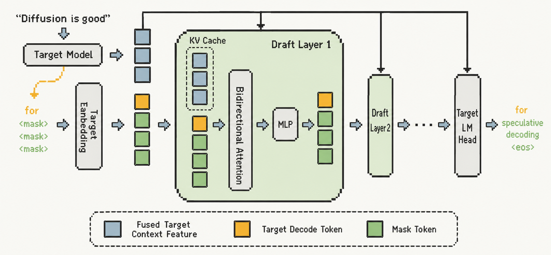
• Input fusion: Gives the draft model target info once at the beginning.
• KV injection: Keeps the target info available inside every draft layer.

How does training look like?

prompt: p1 p2 p3 p4
response: r1 r2 r3 r4 r5 r6 ...

• You pick an anchor token from response.
• Mask the next few tokens

r1 [MASK] [MASK] [MASK]

we try to predict the three mask tokens

x0 x1 x2

• The model learns to predict the masked tokens in parallel. So essentially you get logits for several draft tokens in parallel. For every position k, you get the model’s distribution of what tokens are likely (similar to vanilla LLM inference).

The DFlash implementation: github

We can see how the concepts are implemented (quick example):

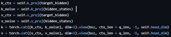
• here we run the target_hidden through the same K/V projection matrices used for draft’s own tokens, concatenating the results into the KV sequence that every query attends over.
• target_hidden in case you didn’t notice is the hidden representation we talked about.

what DSpark brings to the table?

In DSpark, a parallel backbone (DFlash) handles the bulk of draft computation. This keeps $T_{draft}$ nearly independent of $\lambda$. A lightweight sequential block (Markov head + RNN head, we’ll talk more about them soon!) then injects dependency among draft tokens, improving $\tau$ at minimal additional latency.

Recall $\tau$: number of accepted tokens per-cycle

In addition to this, a confidence head estimates per-position acceptance probabilites, and a hardware aware scheduler uses this to get rid of low confidence-suffix tokens.

• Under light load: extra verification token is cheap, it may verify longer prefixes, even if later tokens are somewhat risky.
• Under heavy load: extra verification token is expensive. So shorter prefixes.

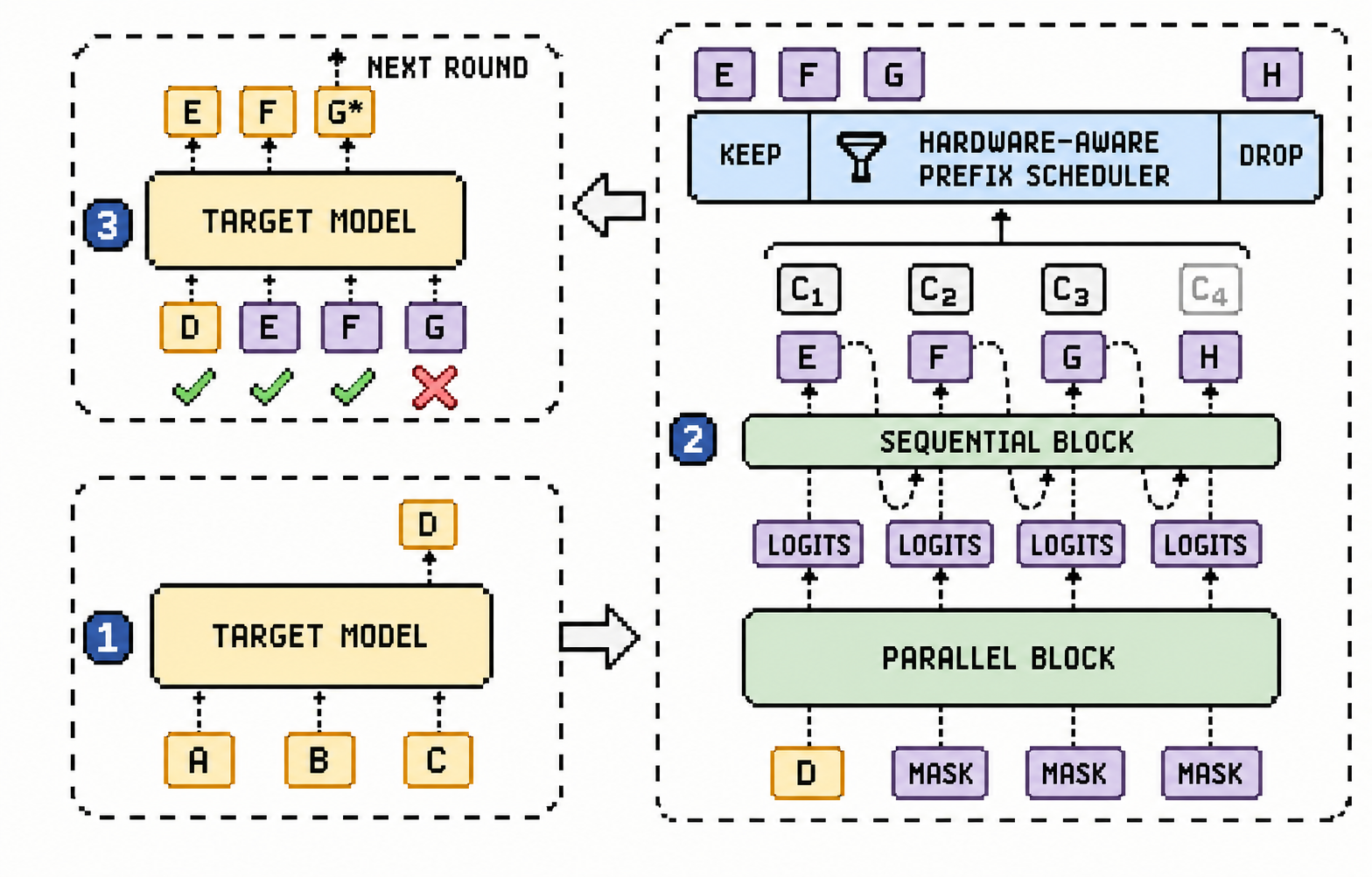
Before we dive deeper into the individual components, let’s organize our mental model:

• Parallel Stage: DFlash; slightly modified.
• Sequential Stage: Somewhat conditions generated tokens on previous one.
• Confidence: Gives us the probability of the token being accepted. Now our scheduler can look at this and the hardware utilization and determine whether it wants to take the chance or not.
• Hardware aware prefix scheduler: Looks at confidence and hardware utilization to determine prefix length (Upto what point shall it accept tokens).

Parallel part

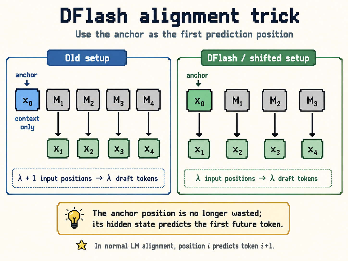
It’s practically DFlash. The only thing that changes is:

Instead of feeding an anchor token and predicting only the mask positions. We treat the anchor itself as the first prediction position. So, $\lambda$ input tokens yield $\lambda$ draft tokens.

Sequential part

Remember the base logits are parallel model generates? (for positon 0, we get a vector containing raw scores for all tokens.) This stage supplements them with a prefix-dependent transition bias $B_{k}$.

what that means essentially is, we add bias to logits and re-normalize and calculate the softmax so on. How we get the bias is what this section is all about.

Now there are two ways to make this sequential head work (get the bias), two different instantiations if you will:

Markov head:

It restricts $B_{k}$ to depend only on the immediately preceding token, reducing it to a first order transition.

Given the preceding token $x_{k-1}$, the transition bias for position k is:

$B(x_{k-1},.)=W1[x_{k-1}]W2$

• In principle it would be a full vocab size x vocab size matrix but that can be very large.
• W1: has V rows, each of length r. For example, Row b is a learned vector that answers “if previous token is b, what does that imply about what comes next?”
• W2: has one row per latent dimension and one column per vocab word (r rows, V columns). Column a answers “how much does each of the r latent factors push this word’s logit up or down?”

self.markov_w1 = nn.Embedding(self.vocab_size, self.markov_rank)
self.markov_w2 = nn.Linear(self.markov_rank, self.vocab_size, bias=False)

• as seen in the source code for dspark. github

return logits + self.compute_step_bias(token_ids, hidden_states)

• it’s added to the logits.

RNN head:

maintains a recurrent state $s_k$ that accumulates the full prefix history within a block.

So at each step, the module concatenates:

• the current state
• the previous token embedding
• backbone hidden state: hidden states are the vectors right before the final vocab projection.

put mathematically:

$z_k​=[s_k−1​;W1​[x_{k−1​}];h_k​]$

z = torch.cat([state, prev_embeddings, hidden_states], dim=-1)
# as seen in the source code. (all the link are available in the reference btw)
proj = self.joint_proj(z)
gate_raw, candidate_raw, output_raw = proj.chunk(3, dim=-1)

then it updates memory using a gate:

$s_k = g_k \odot s_{k-1} + (1 - g_k) \odot \tilde{s}_k$

where:

$g_k = \sigma(W_g z_k)$

$\tilde{s}_k = \tanh(W_c z_k)$

new_state = gate * state + (1.0 - gate) * candidate

This essentially means, if gate is high keep old memory and if it’s low write new memory.

Then, produce the vocab balance: $B_k(x_{<k}, \cdot) = W_2^\top \tanh(W_o z_k),$

bias = self.project_bias(torch.tanh(output_raw))

def project_bias(self, latent_states):
    return self.markov_w2(latent_states)
# markov_w2 maps the small latent vector into a full vocab-sized bias

Finally add bias to the base logits.

Confidence head

This saves us resources by only forwarding tokens with positive expected returns. DSpark couples a confidence head that predicts prefix survival probabilities, with a hardware-aware prefix scheduler.

For each draft position k. $c_{k}$ models the conditional probability (gives a number between 0 and 1) that the draft token at position k will survive target verification, given that all the tokens before in the block have been accepted.

the models estimated prediction of success:

$c_k = \sigma(w^\top[h_k; W_1[x_{k-1}]])$

to supervise confidence heads during traning we use:

$c_k^* = 1 - \frac{1}{2}|p_k^d - p_k^t|_1$

(difference between probability distribution of the draft model and the target model)

Since, we are not using a threshold based approach just knowing a value between 0 and 1 is not enough. We need the absolute magnitudes of the cumulative acceptance probabilites to compute the expected acceptance length.

The paper talks about how raw estimates are often overconfident and would distort our estimation. So they introduce “Sequential temperature scaling” (STS).

survival of prefix up to k = c1 x c2 x … x ck

What STS does:

• Looks at a position and find a single number (Temperature) that you divide with c1’s (say) logit before applying sigmoid.
• It’s chosen so that the resulting c1 matches the empirical survival state we actually observe on the validation set.
• Repeat through position $\lambda$.

Temperature scaling is just squashing/stretching the sigmoid curve. It does not flip the order.

Hardware aware prefix scheduler

The algorithm essentially follows the following steps:

• For every user and every position calculate the prefix survival probabilities.

example: a1 a2 a3
a1=0.83
a2 (a1 a2)=0.61
a3 (a1 a2 a3)=0.32

• Now collect all candidate prefix tokens from all active requests and sort them. Highest would come first obviously.
• Add verification tokens one by one and check throughput
• Stop when adding another token hurts throughput.

How do we know if it would hurt the throughput?

$\Theta = \tau \cdot \mathrm{SPS}(B) $

essentially we would check it before and after adding the token. This is measured beforehand by profiling the engine. So it’s basically a cheap lookup during the actual process.

So how well does it ACTUALLY work?

• They evaulate it on four target models spanning different scales and model families: Qwen3 -(4B, 8B, and 14B) and gemma4-12B.
• DSpark is compared with two representative drafters: DFlash and Eagle3.
• Evaluation protocol:
  • Mathematical reasoning: GSM8K, MATH500, AIME25
  • Code generation: MBPP, HumanEval, Live-CodeBench
  • Daily Chat: MT-Bench, Alpaca and Arena-Hard.
• The specifics are well presented in the paper so I’d encourage you to read that. (All links in the references section)

I’ll just focus on the cool findings:

• Across the Qwen3-4B,8B,and14B models, DSpark improves the macro-average accepted length over Eagle3 by 30.9%, 26.7% and 30.0% respectively.
• Similarly, compared to DFlash, DSpark yields relative improvements of 16.3%, 18.4% and 18.3% across the three scales.
• As shown in the following table: DSpark outperforms the other two at every draft position across all domains:

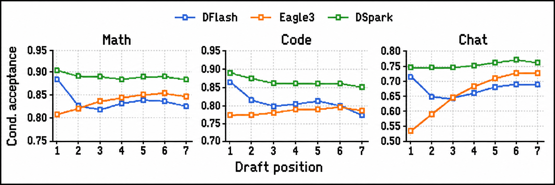
You can also see the rapid acceptance decay in action for DFlash! So basically DSpark inherits high initial acceptance of a deep parallel drafter and simultaneously its sequential head mitigates the decay which is typical of parallel generation.

• A 2-layer DSpark outperforms 5-layer DFlash across all domains!

Where are we headed?

I’m super new to this world of inference optimization, but I do wonder if speedups like DSpark, DFlash, MTP, etc might get us to a point where model spillover to the RAM (CPU) is more tolerable. It may make offloading more practical by giving the system extra time to prefetch/compress/prepare future KV-cache data.

When KV cache is the bottle-neck, this paper (QuantSpec) introduces a pretty cool idea: the draft model shares the architecture of the target model but employs a hierarchical 4-bit quantized KV cache and 4-bit quantized weights for acceleration (haven’t read the paper properly yet).

References

1. DSpark paper
2. DFlash paper
3. Deepseek deepspec repository
4. Z-lab’s DFlash repository